R and RStudio basics

Welcome!

The practical component of the Statistics II: Statistical Modeling and Causal Inference course relies largely in R programming. Today we will center on some of the necessary skills to perform the assignments for the course.

In this tutorial, you will learn to:

• identify the some of the basic functionalities of R and RStudio
• import data sets into your R environment

R and RStudio: Basics

The RStudio layout

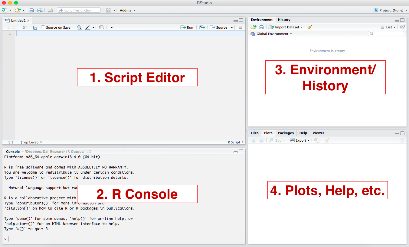
RStudio is an integrated development environment (IDE) for R. Think of RStudio as a front that allows us to interact, compile, and render R code in a more instinctive way. The following image shows what the standard RStudio interface looks like:

1. Console: The console provides a means to interact directly with R. You can type some code at the console and when you press ENTER, R will run that code. Depending on what you type, you may see some output in the console or if you make a mistake, you may get a warning or an error message.

2. Script editor: You will utilize the script editor to complete your assignments. The script editor will be the space where files will be displayed. For example, once you download and open the bi-weekly assignment .Rmd template, it will appear here. The editor is a where you should place code you care about, since the code from the console cannot be saved into a script.

3. Environment: This area holds the abstractions you have created with your code. If you run myresult <- 5+3+2, the myresult object will appear there.

4. Plots and files: This area will be where graphic output will be generated. Additionally, if you write a question mark before any function, (i.e. ?mean) the online documentation will be displayed here.

---

R Packages

For the most part, R Packages are collections of code and functions that leverage R programming to expand on the basic functionalities. Last week we met dplyr that aids R programmers in the process of data cleaning and manipulation. There are a plethora of packages in R designed to facilite the completion of tasks. In fact, this website is built with the blogdown package that lets you create websites using RMarkdown and Hugo

Unlike other programming languages, in R you only need to install a package once. The following times you will only need to “require” the package. As a good practice I recommend running the code to install packages only in your R console, not in the code editor. You can install a package with the following syntax

install.packages("name_of_your_package") #note that the quotation marks are mandatory at this stage

Once the package has been installed, you just need to “call it” every time you want to use it in a file by running:

library("name_of_your_package") #either of this lines will require the package
library(name_of_your_package) #library understands the code with, or without, quotation marks

---

Working directory

The working directory is just a file path on your computer that sets the default location of any files you read into R, or save out of R. Normally, when you open RStudio it will have a default directory (a folder in your computer). You can check you directory by running getwd() in your console:

#this is the default in my case
getwd()
#[1] "/Users/sebastianramirezruiz"

When your RStudio is closed and you open a file from your finder in MacOS or file explorer in Windows, the default working directory will be the folder where the file is hosted

---

Setting your working directory

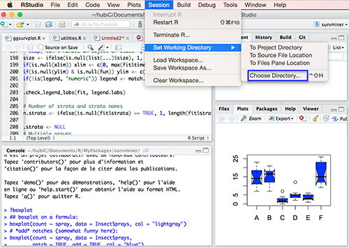
You can set you directory manually from RStudio: use the menu to change your working directory under Session > Set Working Directory > Choose Directory.

You can also use the setwd() function:

setwd("/path/to/your/directory") #in macOS
setwd("c:/path/to/your/directory") #in windows

---

Recommended folder structure for the class

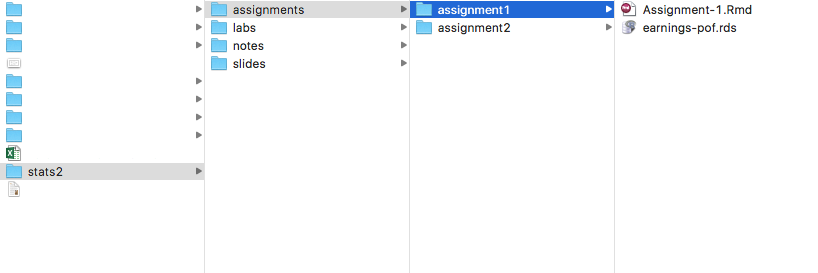
We recommend you pay close attention to your folder structure. You will receive a new folder for each assignment. Make the folder your working directory when working on the assignment. This folder will be populated with the template .Rmd and the data for the week. When you knit the file, the .html will be created in this folder.

---

Dealing with errors in R

Errors in R occur when code is used in a way that it is not intended. For example when you try to add two character strings, you will get the following error:

"hello" + "world"
Error in "hello" + "world": non-numeric argument to binary operator

Normally, when something has gone wrong with your program, R will notify you of an error in the console. There are errors that will prevent the code from running, while others will only produce warning messages. In the following case, the code will run, but you will notice that the string “three” is turned into a NA.

as.numeric(c("1", "2", "three"))
Warning: NAs introduced by coercion
[1]  1  2 NA

Since we will be utilizing widely used packages and functions in the course of the semester, the errors that you may come across in the process of completing your assignments will be common for other R users. Most errors occur because of typos. A Google search of the error message can take you a long way as well. Most of the times the first entry on stackoverflow.com will solve the problem.

---

Importing data

Next we will work with data provided by the palmerpenguins package; however, most practical applications will require you to work with your own data. In fact, for most assignments, you will be given a data set to work with. As we will see in the coming weeks, data are messy. You know what else is messy? Data formats. You may be acquainted with a couple of them (.csv, .tsv, .xlsx).

Fortunately for us, the tidyverse has two packages that make the process of loading data sets from different formats very easy.

• readr: The goal of readr is to provide a fast and friendly way to read rectangular data (like csv, tsv, rds, and fwf)
• haven: The goal of haven is to enable R to read and write various data formats used by other statistical packages (like dta, sas, and sav)

You can read more about how to load different types of data in the respective documentations of the packages — readr and haven

---

For the assignments you will be required to load datasets. You can do that by installing the readr package and utilizing:

#with readr
your_data_frame <- readr::read_rds("path_for_the_file")

#you can alternatively use a base R option
your_data_frame <- base::readRDS("path_for_the_file")

This week’s mock assignment will feature a .tsv file. When in doubt just Google “How to load x_format data in R?" That will do the trick!

---

The double colon operator ::

You may have noted in the previous section that the functions were preceded by their package name and two colons, for example: readr::read_rds(). The double colon operator :: helps us ensure that we select functions from a particular package. We utilize the operator to explicitly state where the function is coming. This may become even more important when you are doing data analysis as part of a team further in your careers. Though it is likely that this will not be a problem during the course, we can try to employ the following convention package_name::function() to ensure that we will not encounter errors in our knitting process:

dplyr::select()

---

Let’s look at what happens when we load tidyverse.

library(tidyverse)

#── Attaching packages ──────────────────────────────────────────────────────────────────────────── tidyverse 1.3.0 #──
#✓ ggplot2 3.3.2     ✓ purrr   0.3.4
#✓ tibble  3.0.3     ✓ dplyr   1.0.2
#✓ tidyr   1.1.2     ✓ stringr 1.4.0
#✓ readr   1.3.1     ✓ forcats 0.5.0
#── Conflicts ─────────────────────────────────────────────────────────────────────────────── tidyverse_conflicts() #──
#x dplyr::filter() masks stats::filter()
#x dplyr::lag()    masks stats::lag()

You may notice that R points out some conflicts where some functions are being masked. The default in this machine will become the filter() from the dplyr package during this session. If you were to run some code that is based on the filter() from the stats package, your code will probably result in errors.

---